3.7 Acceleration-Time Graphs

Definition

An acceleration-time graph displays how the acceleration of an object changes over time. It illustrates the rate of change of velocity during each interval of motion.

Acceleration-time graphs show whether acceleration is constant, changing, or zero.

Reading an Acceleration-Time Graph

In an acceleration-time graph:

• Time t is plotted on the horizontal axis (x-axis) in seconds $(\text{s})$.
• Acceleration a is plotted on the vertical axis (y-axis) in meters per second squared $(\text{m/s}^2)$.

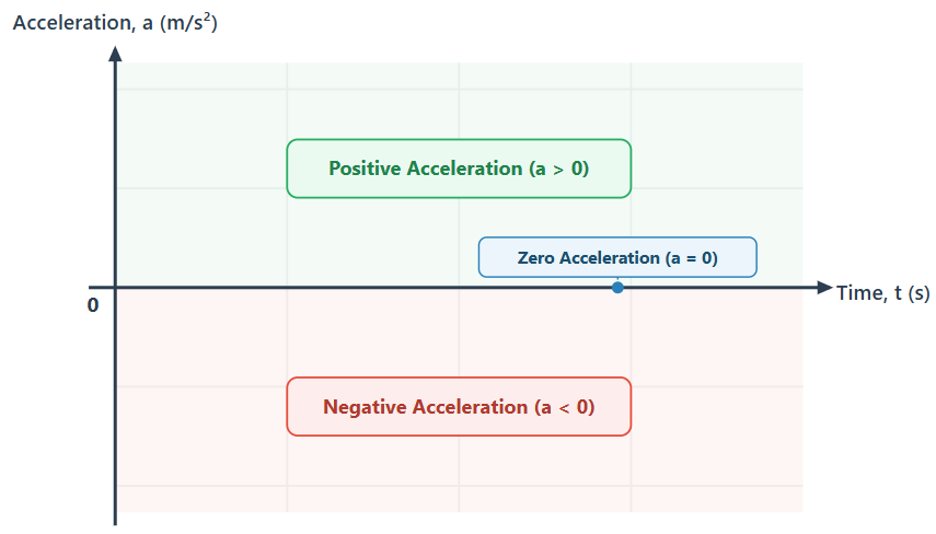
A point above the time axis indicates positive acceleration. A point on the time axis indicates zero acceleration. A point below the time axis indicates negative acceleration.

Zero Acceleration

When the line lies directly on the horizontal axis, the acceleration is zero.

$a = 0$

Zero acceleration means the velocity of the object does not change. The object moves at constant velocity or remains at rest.

Constant Acceleration

In uniform acceleration, the acceleration remains constant over time.

A constant acceleration is represented by a horizontal line parallel to the time axis.

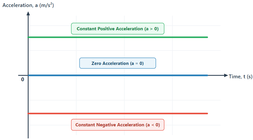
• If the horizontal line is above the time axis, the acceleration is constant and positive.
• If the horizontal line lies on the time axis, the acceleration is zero.
• If the horizontal line is below the time axis, the acceleration is constant and negative.

Area Under an Acceleration-Time Graph

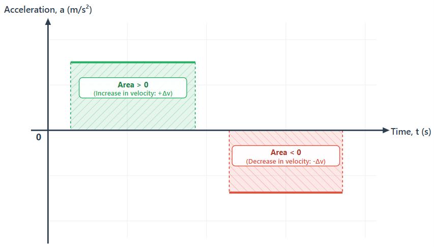
The area under an acceleration-time graph represents the change in velocity $(\Delta v)$ during that time interval.

Because acceleration is the rate of change of velocity:

$a = \frac{\Delta v}{\Delta t}$

Rearranging gives:

$\Delta v = a \Delta t$

On the graph, a corresponds to the height of the rectangle and $\Delta t$ corresponds to the width. Therefore:

$\text{Area} = \Delta v = v_f – v_i$

Where:

• $\Delta v$ is the change in velocity
• $v_f$ is the final velocity
• $v_i$ is the initial velocity
• $a$ is the acceleration
• $\Delta t$ is the time interval

Sign of the Area

• Area above the time axis is positive and represents an increase in velocity.
• Area below the time axis is negative and represents a decrease in velocity.

The total change in velocity is the algebraic sum of all areas:

$\Delta v_{\text{total}} = \text{Area}_{\text{positive}} + \text{Area}_{\text{negative}}$

Important Distinction: The area under an acceleration-time graph does not give the actual velocity at a given instant; it gives only the change in velocity $(\Delta v)$. To determine the final velocity, the initial velocity must be known:

$v_f = v_i + \Delta v$

Example 1: Finding Change in Velocity

A car moves along a straight road with a constant acceleration of $3 \text{ m/s}^2$ for $6 \text{ s}$.

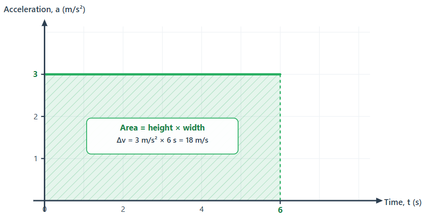
The area under the graph between t = 0 $\text{ s}$ and $t = 6 \text{ s}$ is:

$\Delta v = \text{height} \times \text{width}$

$\Delta v = 3 \text{ m/s}^2 \times 6 \text{ s}$

$\Delta v = 18 \text{ m/s}$

The velocity of the car increases by $18 \text{ m/s}$.

If the car had an initial velocity of $v_i = 5 \text{ m/s}$:

$v_f = v_i + \Delta v$

$v_f = 5 \text{ m/s} + 18 \text{ m/s} = 23 \text{ m/s}$

Example 2: Motion with Positive and Negative Acceleration

An object starts from rest $(v_i = 0)$ and moves according to the following acceleration-time profile:

• Interval 1: $a = 4 \text{ m/s}^2$ from $t = 0 \text{ s}$ to $t = 3 \text{ s}$
• Interval 2: $a = 0 \text{ m/s}^2$ from $t = 3 \text{ s}$ to $t = 7 \text{ s}$
• Interval 3: $a = -2 \text{ m/s}^2$ from $t = 7 \text{ s}$ to $t = 10 \text{ s}$

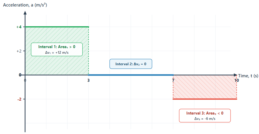
Step 1: Calculate the change in velocity for each interval

For Interval 1:

$\Delta v_1 = 4 \text{ m/s}^2 \times 3 \text{ s} = 12 \text{ m/s}$

For Interval 2:

$\Delta v_2 = 0 \text{ m/s}^2 \times 4 \text{ s} = 0 \text{ m/s}$

For Interval 3:

$\Delta v_3 = -2 \text{ m/s}^2 \times 3 \text{ s} = -6 \text{ m/s}$

Step 2: Determine total change in velocity

$\Delta v_{\text{total}} = 12 \text{ m/s} + 0 \text{ m/s} + (-6 \text{ m/s}) = 6 \text{ m/s}$

Step 3: Determine final velocity

$v_f = v_i + \Delta v_{\text{total}}$

$v_f = 0 \text{ m/s} + 6 \text{ m/s} = 6 \text{ m/s}$

Key Points

• An acceleration-time graph displays acceleration on the vertical axis and time on the horizontal axis.
• A horizontal line parallel to the time axis indicates constant acceleration.
• A line along the time axis represents zero acceleration, meaning constant velocity or rest.
• The area under an acceleration-time graph represents the change in velocity $(\Delta v)$.
• Area above the time axis represents an increase in velocity (positive $\Delta v$).
• Area below the time axis represents a decrease in velocity (negative $\Delta v$).
• To find final velocity, the change in velocity obtained from the area must be added to the initial velocity.