3.8 Equations of Motion

Definition

The equations of motion describe the relationship between displacement, initial velocity, final velocity, acceleration, and time for an object moving in a straight line. These equations apply exclusively to motion under constant (uniform) acceleration. They connect five fundamental kinematic variables.

The Kinematic Variables

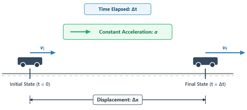
To analyze motion using these equations, five primary variables are defined:

• $\Delta x$: displacement of the object in meters $(\text{m})$
• $v_i$: initial velocity at the start of the time interval in meters per second $(\text{m/s})$
• $v_f$: final velocity at the end of the time interval in meters per second $(\text{m/s})$
• $a$: constant acceleration in meters per second squared $(\text{m/s}^2)$
• $\Delta t$: time elapsed during the motion in seconds $(\text{s})$

Each equation relates four of these five variables, allowing any unknown quantity to be calculated when three variables are known.

Equation 1: Velocity as a Function of Time

The first equation relates final velocity, initial velocity, acceleration, and time:

$v_f = v_i + a \Delta t$

This equation is derived directly from the definition of constant acceleration:

$a = \frac{\Delta v}{\Delta t} = \frac{v_f – v_i}{\Delta t}$

Multiplying both sides by $\Delta t$ and solving for $v_f$ gives the first equation of motion.

Equation 2: Displacement from Average Velocity

When acceleration is constant, velocity changes at a steady rate. The average velocity $v_{\text{avg}}$ during the interval is simply the arithmetic mean of the initial and final velocities:

$v_{\text{avg}} = \frac{v_i + v_f}{2}$

Because displacement is average velocity multiplied by time $(\Delta x = v_{\text{avg}} \Delta t)$, the second equation is:

$\Delta x = \left( \frac{v_i + v_f}{2} \right) \Delta t$

This equation does not require acceleration a to find displacement.

Equation 3: Displacement as a Function of Time

The third equation relates displacement, initial velocity, time, and acceleration:

$\Delta x = v_i \Delta t + \frac{1}{2} a (\Delta t)^2$

Derivation from a Velocity-Time Graph: As shown in Figure 3.8.2, the area under a velocity-time graph represents displacement.

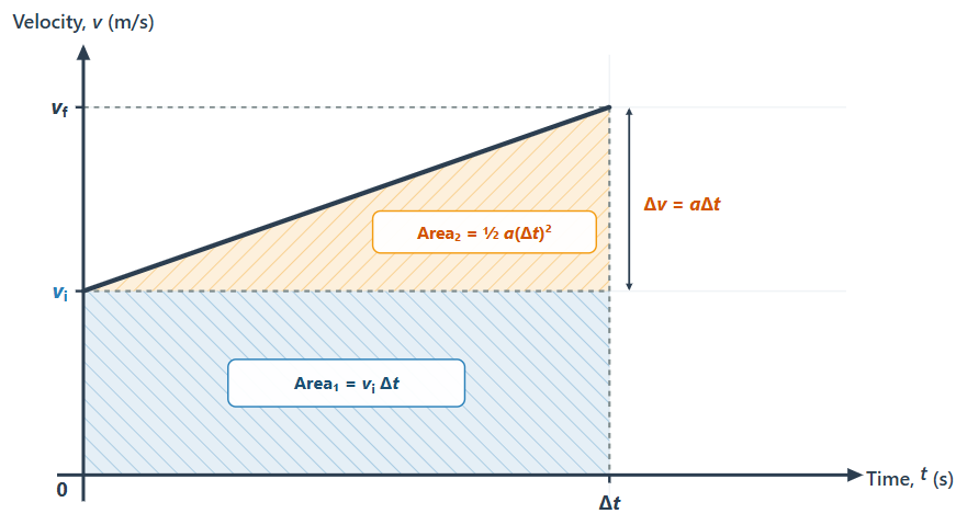
For motion starting at $v_i$and accelerating uniformly to $v_f$, the area under the curve is split into two geometric shapes:

1. A bottom rectangle of height $v_i$ and base $\Delta t$, with area $v_i \Delta t$.
2. A top triangle of base $\Delta t$ and height $\Delta v = a \Delta t$, with area $\frac{1}{2} (\Delta t)(a \Delta t) = \frac{1}{2} a (\Delta t)^2$.

Summing the two areas yields the total displacement.

Equation 4: Velocity as a Function of Position (Time-Independent Equation)

When the elapsed time $\Delta t$ is not known and not required, the time variable can be eliminated by combining Equation 1 and Equation 2:

Solving Equation 1 for time gives:

$\Delta t = \frac{v_f – v_i}{a}$

Substituting this expression into Equation 2:

$\Delta x = \left( \frac{v_f + v_i}{2} \right) \left( \frac{v_f – v_i}{a} \right)$

$\Delta x = \frac{v_f^2 – v_i^2}{2a}$

Rearranging terms yields the fourth kinematic equation:

$v_f^2 = v_i^2 + 2a \Delta x$

Summary Table of the Equations of Motion

Each equation contains four kinematic variables and leaves out exactly one:

• $v_f = v_i + a \Delta t$ (Omits displacement $\Delta x$)
• $\Delta x = \left( \frac{v_i + v_f}{2} \right) \Delta t$ (Omits acceleration $a$)
• $\Delta x = v_i \Delta t + \frac{1}{2} a (\Delta t)^2$ (Omits final velocity $v_f$)
• $v_f^2 = v_i^2 + 2a \Delta x$ (Omits time $\Delta t$)

Example 1: Accelerating Vehicle from Rest

A car starts from rest $(v_i = 0)$ and accelerates uniformly at $2.5 \text{ m/s}^2$ for $8 \text{ s}$ along a straight road. Find the displacement covered by the car and its final velocity.

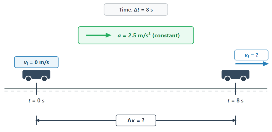
Displacement: To find displacement when final velocity is not required:

$\Delta x = v_i \Delta t + \frac{1}{2} a (\Delta t)^2$

$\Delta x = (0)(8) + \frac{1}{2} (2.5)(8)^2$

$\Delta x = 80 \text{ m}$

Final Velocity: Using the first kinematic equation:

$v_f = v_i + a \Delta t$

$v_f = 0 + (2.5)(8)$

Example 2: Braking Distance (Time-Independent)

A train travels at an initial velocity of $30 \text{ m/s}$. The engineer applies the brakes, producing a constant acceleration of $-1.5 \text{ m/s}^2$ until the train comes to a complete stop. Find the stopping distance of the train.

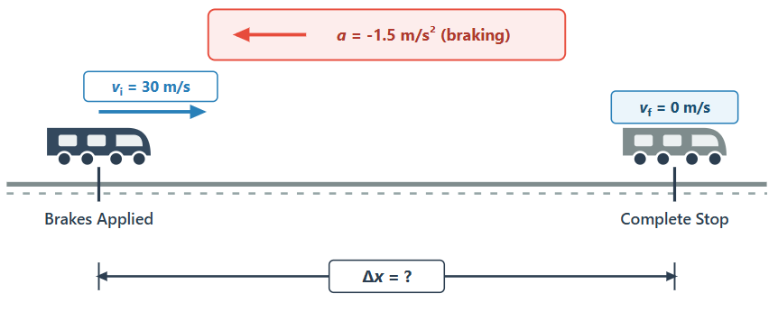
Because time $\Delta t$ is neither given nor requested, use the time-independent equation:

$v_f^2 = v_i^2 + 2a \Delta x$

$0^2 = (30)^2 + 2(-1.5) \Delta x$

$0 = 900 – 3 \Delta x$

$3 \Delta x = 900$

$\Delta x = 300 \text{ m}$

The stopping distance of the train is $300 \text{ m}$.

Key Points

• The equations of motion describe rectilinear motion under strictly constant acceleration.
• There are five primary kinematic variables: displacement $(\Delta x)$, initial velocity $(v_i)$, final velocity $(v_f)$, acceleration $(a)$, and time interval $(\Delta t)$.
• Each kinematic equation relates four variables and omits exactly one.
• The first equation, $v_f = v_i + a \Delta t$, omits displacement and stems from the definition of acceleration.
• The second equation,$\Delta x = \left( \frac{v_i + v_f}{2} \right) \Delta t$, uses average velocity and omits acceleration.
• The third equation, $\Delta x = v_i \Delta t + \frac{1}{2} a (\Delta t)^2$, corresponds to the area under a velocity-time graph and omits final velocity.
• The fourth equation, $v_f^2 = v_i^2 + 2a \Delta x$, relates velocities and displacement independently of time.
• Vector directions must be assigned consistent algebraic signs (positive or negative) before solving.